A Beginner's Guide to Ridge Regression (L2 Regularization)

Introduction

You have learned how to fit a linear regression model that minimizes the sum of squared errors. But what happens when your predictors are highly correlated with each other, for example, house size and number of rooms, which tend to increase together? Or when your dataset is small and noisy?

In these situations, ordinary linear regression often produces coefficients that are unstable and extremely large. The model memorizes the training data too closely (overfitting) and performs poorly on new data it has never seen.

Ridge Regression, also called L2 regularization, is a simple modification to linear regression that fixes this problem by adding a cost to large coefficients. It is one of the most practical and widely used tools in machine learning.

1. Why Does Ordinary Regression Struggle?

Ordinary Least Squares (OLS) regression finds the coefficients by minimizing the sum of squared errors:

J(\beta) = \sum_{i=1}^{n} (y_i - \hat{y}_i)^2

This works well when predictors are independent and the dataset is large. But when predictors are correlated, a subtle problem emerges in the mathematics: the matrix \(X^T X\) (which appears in the solution formula) becomes nearly singular. A singular matrix cannot be inverted, think of it like trying to divide by zero. The result is that small changes in the data cause the coefficients to swing wildly.

A concrete analogy: imagine trying to figure out which of two nearly identical ingredients, say two slightly different types of sugar, changed the taste of a cake. Because they are so similar, any tiny fluctuation in the experiment gets amplified into a huge apparent difference. Correlated predictors do the same thing to regression coefficients.

2. How Ridge Regression Fixes This

Ridge adds a penalty term to the cost function that punishes large coefficients:

J(\beta) = \sum_{i=1}^{n} (y_i - \hat{y}_i)^2 + \lambda \sum_{j=1}^{p} \beta_j^2

The extra term \(\lambda \sum \beta_j^2\) is the L2 penalty, it grows whenever any coefficient gets large. The model is now forced to balance two competing goals: fit the data well (minimize prediction errors) AND keep the coefficients small (minimize the penalty).

The tuning parameter \(\lambda\) (also called "alpha" in scikit-learn) controls the trade-off:

\(\lambda = 0\): Ridge = OLS, no regularization, original behavior.
\(\lambda\) small (e.g. 0.01): slight shrinkage, coefficients barely change.
\(\lambda\) large (e.g. 100): strong shrinkage, all coefficients pushed close to zero.
\(\lambda \to \infty\): all coefficients go to zero, the model predicts the mean for everything (underfitting).

The right value of \(\lambda\) is found through cross-validation, trying many values and picking the one that works best on held-out data.

L1 and L2 norm constraint regions for regularization — **Figure:** L1 (diamond) and L2 (circle) constraint regions. Ridge uses the L2 ball (circle on the right), it shrinks all coefficients smoothly toward zero without setting any to exactly zero. The smooth circular boundary is why Ridge never eliminates features. Source: Nicoguaro / Wikimedia Commons (CC BY 4.0)

3. The Ridge Solution Formula

The OLS closed-form solution is:

\hat{\beta}_{\text{OLS}} = (X^T X)^{-1} X^T y

For Ridge, minimizing the penalized cost function leads to a modified formula. Taking the derivative and setting it to zero gives:

(X^T X + \lambda I)\beta = X^T y

Solving for \(\beta\):

\hat{\beta}_{\text{ridge}} = (X^T X + \lambda I)^{-1} X^T y

The key difference is \(+ \lambda I\): we add \(\lambda\) to the diagonal of the matrix before inverting. This is guaranteed to make the matrix invertible (no matter how correlated the predictors are), which is exactly what stabilizes the solution.

4. Manual Example (Step by Step)

Let us walk through a tiny numerical example so the formula becomes concrete.

x	y
1	2
2	3
3	5
4	7

We use \(\lambda = 1\) for this example.

Step 1. Build the design matrix \(X\) with an intercept column:

X = \begin{bmatrix}1 & 1 \\ 1 & 2 \\ 1 & 3 \\ 1 & 4 \end{bmatrix}, \quad y = \begin{bmatrix}2 \\ 3 \\ 5 \\ 7\end{bmatrix}

The first column of ones allows the model to estimate an intercept (\(\beta_0\)).

Step 2. Compute \(X^T X\) and \(X^T y\):

X^T X = \begin{bmatrix}4 & 10 \\ 10 & 30\end{bmatrix}, \quad X^T y = \begin{bmatrix}17 \\ 51\end{bmatrix}

Step 3. Add the penalty (\(\lambda I\)):

X^T X + \lambda I = \begin{bmatrix}5 & 10 \\ 10 & 31\end{bmatrix}

Step 4. Invert the modified matrix:

(X^T X + \lambda I)^{-1} = \frac{1}{55}\begin{bmatrix}31 & -10 \\ -10 & 5\end{bmatrix}

Step 5. Multiply to get coefficients:

\begin{bmatrix}31 & -10 \\ -10 & 5\end{bmatrix} \begin{bmatrix}17 \\ 51\end{bmatrix} = \begin{bmatrix}935 - 510 \\ -170 + 255\end{bmatrix} = \begin{bmatrix}425 \\ 85\end{bmatrix}

\hat{\beta}_{\text{ridge}} = \frac{1}{55}\begin{bmatrix}425 \\ 85\end{bmatrix} = \begin{bmatrix}7.727 \\ 1.545\end{bmatrix}

The final model is:

\hat{y} = 7.727 + 1.545x

Compare this to the OLS solution (without Ridge), the intercept and slope would be slightly different because Ridge shrinks both toward zero. The larger \(\lambda\), the more shrinkage.

5. Manual Calculation in Python (NumPy)


import numpy as np

# Design matrix with intercept column
X = np.array([[1,1],[1,2],[1,3],[1,4]])
y = np.array([2,3,5,7])
lmbda = 1

XtX = X.T @ X
Xty = X.T @ y
ridge_matrix = XtX + lmbda * np.eye(XtX.shape[0])  # Add lambda * I
ridge_inv = np.linalg.inv(ridge_matrix)
beta_ridge = ridge_inv @ Xty

print("Ridge coefficients:", beta_ridge)
# Output: [7.727, 1.545]

6. Ridge in Scikit-learn


from sklearn.linear_model import Ridge
import numpy as np

X_feature = np.array([[1],[2],[3],[4]])
y = np.array([2,3,5,7])

# alpha in scikit-learn corresponds to lambda in the formula
ridge = Ridge(alpha=1, fit_intercept=True)
ridge.fit(X_feature, y)

print("Intercept:", ridge.intercept_)
print("Coefficient:", ridge.coef_)

7. Visualizing the Ridge Effect

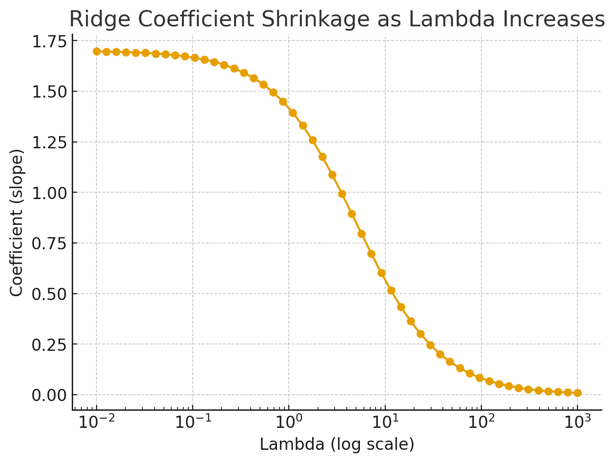
Coefficients vs \(\lambda\)

As \(\lambda\) increases from left to right, all coefficients are progressively squeezed toward zero. Crucially, they never reach exactly zero. Ridge shrinks but does not eliminate. This is Ridge's defining characteristic, and it differs fundamentally from Lasso (covered in the next post).

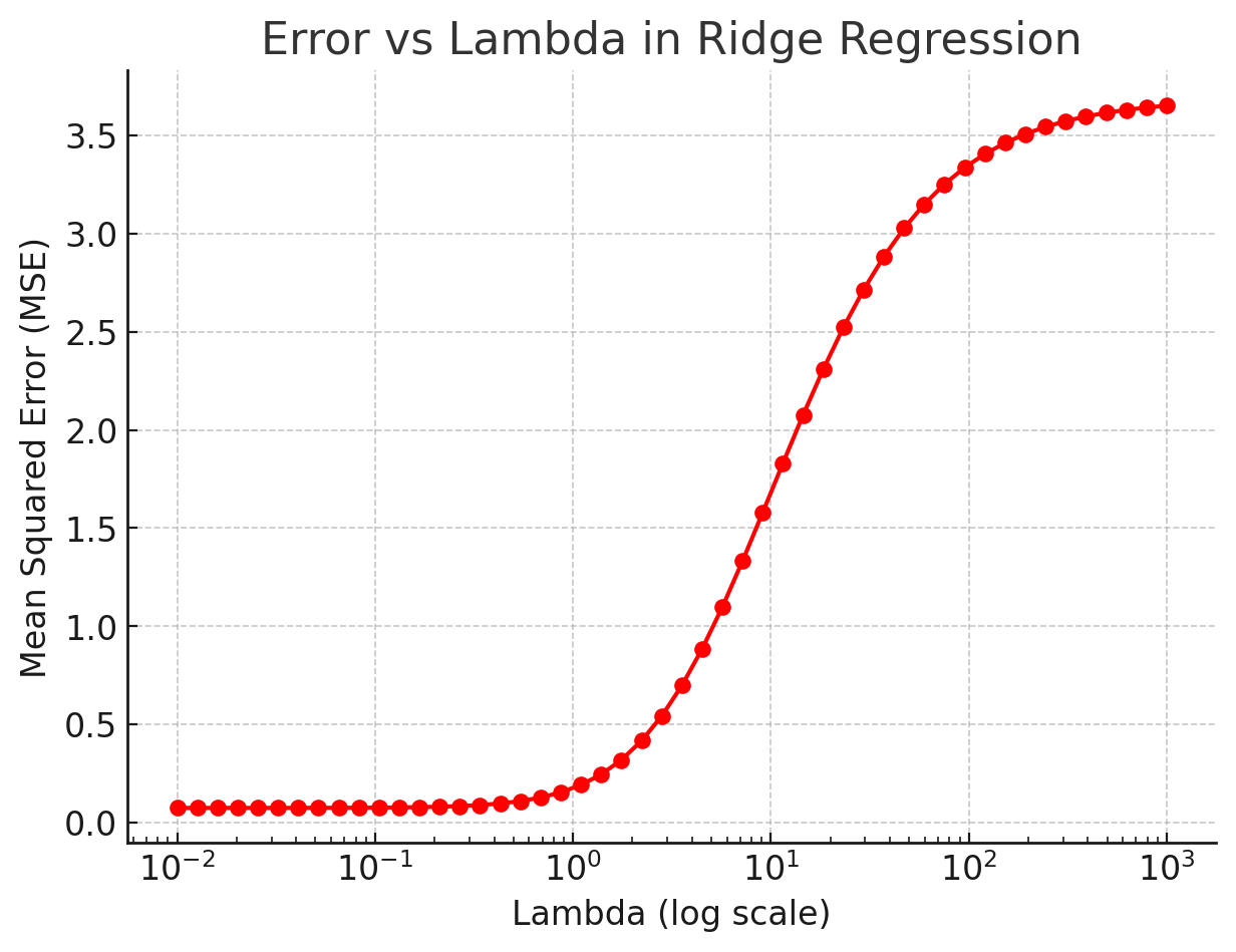
Ridge regression coefficients shrinking toward zero as lambda increases — **Figure:** Each line is one coefficient's value as λ grows. Ridge shrinks all of them smoothly toward zero but never to exactly zero, no feature is completely removed.

Error vs \(\lambda\) (The Bias-Variance Tradeoff)

This plot shows training error and validation error as \(\lambda\) changes. It illustrates one of the most important concepts in machine learning: the bias-variance tradeoff.

Very small \(\lambda\) → model is complex, fits training data perfectly (overfitting), but fails on new data.
Very large \(\lambda\) → model is too simple, coefficients all shrink to near-zero (underfitting).
The sweet spot minimizes validation error, found using cross-validation.

Training and validation error vs lambda showing the bias-variance tradeoff — **Figure:** Training error (low side) and validation error form a U-shape as λ grows. The optimal λ sits at the bottom of the validation error curve.

8. When Should You Use Ridge?

When several of your features are correlated (multicollinearity). Ridge stabilizes the estimates.
When you have more features than observations. OLS breaks down, Ridge handles this gracefully.
When you want to reduce overfitting on noisy data without eliminating any features.
When you care more about prediction accuracy than the exact value of individual coefficients.

9. Pros and Cons

Strengths

Stabilizes regression when predictors are correlated.
Improves prediction accuracy on unseen data by reducing overfitting.
Always mathematically solvable, the added \(\lambda I\) guarantees invertibility.
Easy to implement and widely supported in all major ML libraries.

Limitations

Does not perform feature selection, coefficients shrink but never reach exactly zero. If you want to identify and remove irrelevant features, use Lasso instead.
Requires tuning \(\lambda\), the right value must be found via cross-validation.
Features must be on the same scale, always standardize your features before applying Ridge, otherwise the penalty treats large-scale features unfairly.

10. Key Takeaways

Ridge adds an L2 penalty (sum of squared coefficients) to the loss function, pushing coefficients toward zero.
It stabilizes models that suffer from correlated predictors or too many features.
\(\lambda\) controls the amount of shrinkage, larger \(\lambda\) means more regularization.
Ridge shrinks all coefficients but never sets any to exactly zero, it is not a feature selector.
Always standardize features and tune \(\lambda\) with cross-validation.